Lec 12 - Split-apply-combine paradigm

Split

Create ‘groups’ or ‘splits’ of the data, for instance:

• along groups based on some categorical variables
• along rolling windows for timeseries data

Apply (aggregate, transform, filter)

• Aggregation: compute a summary statistic (or statistics) for each group.
  → Compute group sums or means, or size/counts within each groups

• Transformation: perform some group-specific computations and return a like-indexed object. Some examples:
  → Standardize data (zscore or subtracting the min and dividing by max-min) within a group.
  → Filling NAs within groups with a value derived from each group (e.g., the mean within the group)

• Filtration: discard some groups, according to a group-wise computation that evaluates to True or False. Some examples:
  → Discard data that belong to groups with fewver than 10 rows.
  → Filter out groups that have more than 30% of missing data.

Combine

After the aggregation, transformation or filtration is done, combine the data back together as one:

• Combine the aggregated summary statistics of all groups in a pivot table
• Combine the transformed columns back into a data-frame of the same length as the original one
• After a filtration, get back the original data, with the filtered out rows discarded

import pandas as pd
import numpy as np
import matplotlib.pyplot as plt
import seaborn as sns

df = pd.read_csv('rates.csv')
df.index = df['Time'].astype(np.dtype('datetime64[ns]'))
df = df.drop(columns='Time')
df = df.sort_index()
df.head()

	USD	JPY	BGN	CZK	DKK	GBP	CHF
Time
2024-01-18	1.0875	160.89	1.9558	24.734	7.4571	0.85773	0.9432
2024-01-19	1.0887	161.17	1.9558	24.813	7.4575	0.85825	0.9459
2024-01-22	1.0890	160.95	1.9558	24.758	7.4585	0.85575	0.9458
2024-01-23	1.0872	160.88	1.9558	24.824	7.4574	0.85493	0.9446
2024-01-24	1.0905	160.46	1.9558	24.786	7.4568	0.85543	0.9415

Row or column-wise function application

df.apply(...) with functions returning scalars (“reduce”)

df.apply('mean')

USD      1.082711
JPY    162.195484
BGN      1.955800
CZK     25.199081
DKK      7.456484
GBP      0.855201
CHF      0.957208
dtype: float64

f = lambda x: (x+1)**2
f(3)

16

# lambda is a quick way to construct a function, usually in one line
df.apply(lambda col: np.mean(col)/np.std(col))

USD    1.615824e+02
JPY    1.007120e+02
BGN    4.404070e+15
CZK    1.151246e+02
DKK    3.479387e+03
GBP    5.131824e+02
CHF    6.359713e+01
dtype: float64

df.apply(...) with functions returning Series (“broadcast)

# centering and normalizing
df.apply(lambda col: (col - np.mean(col)) / col.std(), axis=0)

	USD	JPY	BGN	CZK	DKK	GBP	CHF
Time
2024-01-18	0.708874	-0.804050	0.991903	-2.107564	0.285174	1.505410	-0.923163
2024-01-19	0.886510	-0.631598	0.991903	-1.749567	0.470313	1.814921	-0.745227
2024-01-22	0.930919	-0.767096	0.991903	-1.998805	0.933160	0.326887	-0.751817
2024-01-23	0.664465	-0.810209	0.991903	-1.699719	0.424028	-0.161188	-0.830900
2024-01-24	1.152964	-1.068888	0.991903	-1.871920	0.146319	0.136419	-1.035197
...	...	...	...	...	...	...	...
2024-04-10	0.486828	1.659558	0.991903	0.765476	1.349722	-0.030241	1.567942
2024-04-11	-1.452368	1.222268	0.991903	0.874235	1.812570	0.029281	1.416367
2024-04-12	-2.592200	0.594048	0.991903	0.624997	1.766285	-0.571885	0.948461
2024-04-15	-2.532988	1.142200	0.991903	0.566086	1.905139	-0.684975	1.007773
2024-04-16	-2.814246	1.443993	0.991903	0.049482	2.043993	-0.476651	0.922100

62 rows × 7 columns

df.loc['2023-11-07', 'USD'] = pd.NA
df.loc['2023-11-08', 'JPY'] = pd.NA
df.loc['2023-11-06', 'BGN'] = pd.NA
df.loc['2023-11-09', 'BGN'] = pd.NA
df.head()

	USD	JPY	BGN	CZK	DKK	GBP	CHF
Time
2024-01-18	1.0875	160.89	1.9558	24.734	7.4571	0.85773	0.9432
2024-01-19	1.0887	161.17	1.9558	24.813	7.4575	0.85825	0.9459
2024-01-22	1.0890	160.95	1.9558	24.758	7.4585	0.85575	0.9458
2024-01-23	1.0872	160.88	1.9558	24.824	7.4574	0.85493	0.9446
2024-01-24	1.0905	160.46	1.9558	24.786	7.4568	0.85543	0.9415

df.apply(pd.Series.interpolate).head()

	USD	JPY	BGN	CZK	DKK	GBP	CHF
Time
2024-01-18	1.0875	160.89	1.9558	24.734	7.4571	0.85773	0.9432
2024-01-19	1.0887	161.17	1.9558	24.813	7.4575	0.85825	0.9459
2024-01-22	1.0890	160.95	1.9558	24.758	7.4585	0.85575	0.9458
2024-01-23	1.0872	160.88	1.9558	24.824	7.4574	0.85493	0.9446
2024-01-24	1.0905	160.46	1.9558	24.786	7.4568	0.85543	0.9415

Aggregation API: several .apply at once

.agg with a single function is equivalent to apply

df.agg('mean')

USD      1.082711
JPY    162.195484
BGN      1.955800
CZK     25.199081
DKK      7.456484
GBP      0.855201
CHF      0.957208
dtype: float64

df.agg('mean') - df.apply('mean')

USD    0.0
JPY    0.0
BGN    0.0
CZK    0.0
DKK    0.0
GBP    0.0
CHF    0.0
dtype: float64

def maximum_plus_two(col):
    return col.max() + 2

df.agg(['mean',
        'median',
        lambda col: col.max(),
        maximum_plus_two
       ])

	USD	JPY	BGN	CZK	DKK	GBP	CHF
mean	1.082711	162.195484	1.9558	25.199081	7.456484	0.855201	0.957208
median	1.083900	162.150000	1.9558	25.297000	7.456500	0.855125	0.956150
<lambda>	1.093900	164.970000	1.9558	25.460000	7.460900	0.858460	0.984600
maximum_plus_two	3.093900	166.970000	3.9558	27.460000	9.460900	2.858460	2.984600

df.agg(['mean',
        'median',
        lambda col: col.max(),
        maximum_plus_two
       ], axis=1) # here applying this aggregation functions to rows does not really make sense

/home/pierro/mambaforge/lib/python3.10/site-packages/numpy/lib/nanfunctions.py:1215: RuntimeWarning:

Mean of empty slice

/home/pierro/mambaforge/lib/python3.10/site-packages/numpy/lib/nanfunctions.py:1215: RuntimeWarning:

Mean of empty slice

/home/pierro/mambaforge/lib/python3.10/site-packages/numpy/lib/nanfunctions.py:1215: RuntimeWarning:

Mean of empty slice

/home/pierro/mambaforge/lib/python3.10/site-packages/numpy/lib/nanfunctions.py:1215: RuntimeWarning:

Mean of empty slice

	mean	median	<lambda>	maximum_plus_two
Time
2024-01-18	28.275047	1.9558	160.89	162.89
2024-01-19	28.327021	1.9558	161.17	163.17
2024-01-22	28.287550	1.9558	160.95	162.95
2024-01-23	28.286276	1.9558	160.88	162.88
2024-01-24	28.220861	1.9558	160.46	162.46
...	...	...	...	...
2024-04-16	28.865143	1.9558	164.54	166.54
2023-11-07	NaN	NaN	NaN	NaN
2023-11-08	NaN	NaN	NaN	NaN
2023-11-06	NaN	NaN	NaN	NaN
2023-11-09	NaN	NaN	NaN	NaN

66 rows × 4 columns

Different aggregation functions to different columns

df.agg({"USD": ["mean", "median"],
        "JPY": "sum"})

	USD	JPY
mean	1.082711	NaN
median	1.083900	NaN
sum	NaN	10056.12

penguins = sns.load_dataset("penguins")
penguins.agg({'body_mass_g': ['mean', 'std'],
              'sex': 'unique'})

	body_mass_g	sex
mean	4201.754386	NaN
std	801.954536	NaN
unique	NaN	[Male, Female, nan]

Custom .describe

from functools import partial
q_05 = partial(pd.Series.quantile, q=0.05)
q_05.__name__ = "05%"
q_95 = partial(pd.Series.quantile, q=0.95)
q_95.__name__ = "95%"
df.agg(["count", "mean", "std", "min", q_05, "median", q_95, "max"])

	USD	JPY	BGN	CZK	DKK	GBP	CHF
count	62.000000	62.000000	6.200000e+01	62.000000	62.000000	62.000000	62.000000
mean	1.082711	162.195484	1.955800e+00	25.199081	7.456484	0.855201	0.957208
std	0.006755	1.623635	2.238572e-16	0.220672	0.002161	0.001680	0.015174
min	1.063700	158.960000	1.955800e+00	24.734000	7.453600	0.850980	0.931500
05%	1.071380	159.710500	1.955800e+00	24.759400	7.453905	0.852504	0.934705
median	1.083900	162.150000	1.955800e+00	25.297000	7.456500	0.855125	0.956150
95%	1.092455	164.682500	1.955800e+00	25.414800	7.460395	0.857946	0.981000
max	1.093900	164.970000	1.955800e+00	25.460000	7.460900	0.858460	0.984600

Transform API

The transform() method returns an object that is indexed the same (same size) as the original

df.transform(np.abs)

	USD	JPY	BGN	CZK	DKK	GBP	CHF
Time
2024-01-18	1.0875	160.89	1.9558	24.734	7.4571	0.85773	0.9432
2024-01-19	1.0887	161.17	1.9558	24.813	7.4575	0.85825	0.9459
2024-01-22	1.0890	160.95	1.9558	24.758	7.4585	0.85575	0.9458
2024-01-23	1.0872	160.88	1.9558	24.824	7.4574	0.85493	0.9446
2024-01-24	1.0905	160.46	1.9558	24.786	7.4568	0.85543	0.9415
...	...	...	...	...	...	...	...
2024-04-16	1.0637	164.54	1.9558	25.210	7.4609	0.85440	0.9712
2023-11-07	NaN	NaN	NaN	NaN	NaN	NaN	NaN
2023-11-08	NaN	NaN	NaN	NaN	NaN	NaN	NaN
2023-11-06	NaN	NaN	NaN	NaN	NaN	NaN	NaN
2023-11-09	NaN	NaN	NaN	NaN	NaN	NaN	NaN

66 rows × 7 columns

df.transform(lambda col: np.mean(col)) # error: must conserve same index as the original

ValueError: Function did not transform

df.transform(lambda col: col - np.mean(col))

	USD	JPY	BGN	CZK	DKK	GBP	CHF
Time
2024-01-18	0.004789	-1.305484	-2.220446e-16	-0.465081	0.000616	0.002529	-0.014008
2024-01-19	0.005989	-1.025484	-2.220446e-16	-0.386081	0.001016	0.003049	-0.011308
2024-01-22	0.006289	-1.245484	-2.220446e-16	-0.441081	0.002016	0.000549	-0.011408
2024-01-23	0.004489	-1.315484	-2.220446e-16	-0.375081	0.000916	-0.000271	-0.012608
2024-01-24	0.007789	-1.735484	-2.220446e-16	-0.413081	0.000316	0.000229	-0.015708
...	...	...	...	...	...	...	...
2024-04-16	-0.019011	2.344516	-2.220446e-16	0.010919	0.004416	-0.000801	0.013992
2023-11-07	NaN	NaN	NaN	NaN	NaN	NaN	NaN
2023-11-08	NaN	NaN	NaN	NaN	NaN	NaN	NaN
2023-11-06	NaN	NaN	NaN	NaN	NaN	NaN	NaN
2023-11-09	NaN	NaN	NaN	NaN	NaN	NaN	NaN

66 rows × 7 columns

def norm_mean_std(col):
    return (col - col.mean())/col.std()

def norm_min_max(col):
    return (col - col.min())/(col.max() - col.min())

df.transform([norm_mean_std, norm_min_max])

	USD		JPY		BGN		CZK		DKK		GBP		CHF
	norm_mean_std	norm_min_max	norm_mean_std	norm_min_max	norm_mean_std	norm_min_max	norm_mean_std	norm_min_max	norm_mean_std	norm_min_max	norm_mean_std	norm_min_max	norm_mean_std	norm_min_max
Time
2024-01-18	0.708874	0.788079	-0.804050	0.321131	-0.991903	NaN	-2.107564	0.000000	0.285174	0.479452	1.505410	0.902406	-0.923163	0.220339
2024-01-19	0.886510	0.827815	-0.631598	0.367720	-0.991903	NaN	-1.749567	0.108815	0.470313	0.534247	1.814921	0.971925	-0.745227	0.271186
2024-01-22	0.930919	0.837748	-0.767096	0.331115	-0.991903	NaN	-1.998805	0.033058	0.933160	0.671233	0.326887	0.637701	-0.751817	0.269303
2024-01-23	0.664465	0.778146	-0.810209	0.319468	-0.991903	NaN	-1.699719	0.123967	0.424028	0.520548	-0.161188	0.528075	-0.830900	0.246704
2024-01-24	1.152964	0.887417	-1.068888	0.249584	-0.991903	NaN	-1.871920	0.071625	0.146319	0.438356	0.136419	0.594920	-1.035197	0.188324
...	...	...	...	...	...	...	...	...	...	...	...	...	...	...
2024-04-16	-2.814246	0.000000	1.443993	0.928453	-0.991903	NaN	0.049482	0.655647	2.043993	1.000000	-0.476651	0.457219	0.922100	0.747646
2023-11-07	NaN	NaN	NaN	NaN	NaN	NaN	NaN	NaN	NaN	NaN	NaN	NaN	NaN	NaN
2023-11-08	NaN	NaN	NaN	NaN	NaN	NaN	NaN	NaN	NaN	NaN	NaN	NaN	NaN	NaN
2023-11-06	NaN	NaN	NaN	NaN	NaN	NaN	NaN	NaN	NaN	NaN	NaN	NaN	NaN	NaN
2023-11-09	NaN	NaN	NaN	NaN	NaN	NaN	NaN	NaN	NaN	NaN	NaN	NaN	NaN	NaN

66 rows × 14 columns

df.transform({'USD': [norm_min_max, norm_mean_std],
              'JPY': norm_min_max})

	USD		JPY
	norm_min_max	norm_mean_std	norm_min_max
Time
2024-01-18	0.788079	0.708874	0.321131
2024-01-19	0.827815	0.886510	0.367720
2024-01-22	0.837748	0.930919	0.331115
2024-01-23	0.778146	0.664465	0.319468
2024-01-24	0.887417	1.152964	0.249584
...	...	...	...
2024-04-16	0.000000	-2.814246	0.928453
2023-11-07	NaN	NaN	NaN
2023-11-08	NaN	NaN	NaN
2023-11-06	NaN	NaN	NaN
2023-11-09	NaN	NaN	NaN

66 rows × 3 columns

df[['USD', 'JPY']].transform([norm_min_max, norm_mean_std])

	USD		JPY
	norm_min_max	norm_mean_std	norm_min_max	norm_mean_std
Time
2024-01-18	0.788079	0.708874	0.321131	-0.804050
2024-01-19	0.827815	0.886510	0.367720	-0.631598
2024-01-22	0.837748	0.930919	0.331115	-0.767096
2024-01-23	0.778146	0.664465	0.319468	-0.810209
2024-01-24	0.887417	1.152964	0.249584	-1.068888
...	...	...	...	...
2024-04-16	0.000000	-2.814246	0.928453	1.443993
2023-11-07	NaN	NaN	NaN	NaN
2023-11-08	NaN	NaN	NaN	NaN
2023-11-06	NaN	NaN	NaN	NaN
2023-11-09	NaN	NaN	NaN	NaN

66 rows × 4 columns

Transforming only specific columns with certain functions

df.transform({'USD': [norm_mean_std, 
                      norm_min_max],
              'JPY': np.abs}).head(9)

	USD		JPY
	norm_mean_std	norm_min_max	absolute
Time
2024-01-18	0.708874	0.788079	160.89
2024-01-19	0.886510	0.827815	161.17
2024-01-22	0.930919	0.837748	160.95
2024-01-23	0.664465	0.778146	160.88
2024-01-24	1.152964	0.887417	160.46
2024-01-25	0.975328	0.847682	160.81
2024-01-26	0.649662	0.774834	160.62
2024-01-29	-0.060883	0.615894	160.13
2024-01-30	0.279586	0.692053	159.97

Entry-wise application of arbitrary functions with .map

# entry-wise function application
df.USD.map(lambda u: "more than 1" if u>1 else "less than 1") # convert entries to string

Time
2024-01-18    more than 1
2024-01-19    more than 1
2024-01-22    more than 1
2024-01-23    more than 1
2024-01-24    more than 1
                 ...     
2024-04-16    more than 1
2023-11-07    less than 1
2023-11-08    less than 1
2023-11-06    less than 1
2023-11-09    less than 1
Name: USD, Length: 66, dtype: object

# convert to string and replace dot with the text -DOT-
df.USD.map(lambda u: str(u).replace('.', '-DOT-')) 

Time
2024-01-18    1-DOT-0875
2024-01-19    1-DOT-0887
2024-01-22     1-DOT-089
2024-01-23    1-DOT-0872
2024-01-24    1-DOT-0905
                 ...    
2024-04-16    1-DOT-0637
2023-11-07           nan
2023-11-08           nan
2023-11-06           nan
2023-11-09           nan
Name: USD, Length: 66, dtype: object

Rolling and expanding windows

Rolling windows

df = pd.read_csv('rates.csv')
df.index = df['Time'].astype(np.dtype('datetime64[ns]'))
df = df.drop(columns='Time')
df = df.sort_index()
df.head()

	USD	JPY	BGN	CZK	DKK	GBP	CHF
Time
2024-01-18	1.0875	160.89	1.9558	24.734	7.4571	0.85773	0.9432
2024-01-19	1.0887	161.17	1.9558	24.813	7.4575	0.85825	0.9459
2024-01-22	1.0890	160.95	1.9558	24.758	7.4585	0.85575	0.9458
2024-01-23	1.0872	160.88	1.9558	24.824	7.4574	0.85493	0.9446
2024-01-24	1.0905	160.46	1.9558	24.786	7.4568	0.85543	0.9415

df.rolling(window=3).std()

	USD	JPY	BGN	CZK	DKK	GBP	CHF
Time
2024-01-18	NaN	NaN	NaN	NaN	NaN	NaN	NaN
2024-01-19	NaN	NaN	NaN	NaN	NaN	NaN	NaN
2024-01-22	0.000794	0.147422	0.0	0.040501	0.000721	0.001319	0.001531
2024-01-23	0.000964	0.151327	0.0	0.035360	0.000608	0.001729	0.000723
2024-01-24	0.001652	0.265016	0.0	0.033126	0.000862	0.000413	0.002219
...	...	...	...	...	...	...	...
2024-04-10	0.002364	0.291433	0.0	0.013013	0.000306	0.001401	0.000624
2024-04-11	0.007773	0.434856	0.0	0.012000	0.000721	0.000827	0.001650
2024-04-12	0.010516	0.869617	0.0	0.027574	0.000551	0.000557	0.004900
2024-04-15	0.004335	0.555188	0.0	0.036097	0.000153	0.000645	0.003866
2024-04-16	0.001002	0.699595	0.0	0.069874	0.000300	0.000175	0.000666

62 rows × 7 columns

df.rolling(window=3, min_periods=2).sum()

	USD	JPY	BGN	CZK	DKK	GBP	CHF
Time
2024-01-18	NaN	NaN	NaN	NaN	NaN	NaN	NaN
2024-01-19	2.1762	322.06	3.9116	49.547	14.9146	1.71598	1.8891
2024-01-22	3.2652	483.01	5.8674	74.305	22.3731	2.57173	2.8349
2024-01-23	3.2649	483.00	5.8674	74.395	22.3734	2.56893	2.8363
2024-01-24	3.2667	482.29	5.8674	74.368	22.3727	2.56611	2.8319
...	...	...	...	...	...	...	...
2024-04-10	3.2550	494.29	5.8674	76.102	22.3772	2.56973	2.9436
2024-04-11	3.2456	494.04	5.8674	76.140	22.3788	2.56703	2.9416
2024-04-12	3.2241	492.23	5.8674	76.097	22.3801	2.56464	2.9313
2024-04-15	3.2037	491.39	5.8674	76.053	22.3813	2.56354	2.9228
2024-04-16	3.1945	491.75	5.8674	75.871	22.3818	2.56269	2.9153

62 rows × 7 columns

df.rolling(window=5, center=True).mean()

	USD	JPY	BGN	CZK	DKK	GBP	CHF
Time
2024-01-18	NaN	NaN	NaN	NaN	NaN	NaN	NaN
2024-01-19	NaN	NaN	NaN	NaN	NaN	NaN	NaN
2024-01-22	1.08858	160.870	1.9558	24.7830	7.45746	0.856418	0.94420
2024-01-23	1.08894	160.854	1.9558	24.7874	7.45724	0.855948	0.94396
2024-01-24	1.08862	160.744	1.9558	24.7744	7.45672	0.855034	0.94270
...	...	...	...	...	...	...	...
2024-04-10	1.07862	164.326	1.9558	25.3662	7.45958	0.855844	0.97878
2024-04-11	1.07528	164.250	1.9558	25.3602	7.45994	0.855064	0.97714
2024-04-12	1.07068	164.164	1.9558	25.3262	7.46032	0.854618	0.97500
2024-04-15	NaN	NaN	NaN	NaN	NaN	NaN	NaN
2024-04-16	NaN	NaN	NaN	NaN	NaN	NaN	NaN

62 rows × 7 columns

Expanding windows (cumulative since the start)

df.expanding().max() # useful to compute the highest exchange rate so far since 2023-11-06

	USD	JPY	BGN	CZK	DKK	GBP	CHF
Time
2024-01-18	1.0875	160.89	1.9558	24.734	7.4571	0.85773	0.9432
2024-01-19	1.0887	161.17	1.9558	24.813	7.4575	0.85825	0.9459
2024-01-22	1.0890	161.17	1.9558	24.813	7.4585	0.85825	0.9459
2024-01-23	1.0890	161.17	1.9558	24.824	7.4585	0.85825	0.9459
2024-01-24	1.0905	161.17	1.9558	24.824	7.4585	0.85825	0.9459
...	...	...	...	...	...	...	...
2024-04-10	1.0939	164.97	1.9558	25.460	7.4605	0.85846	0.9846
2024-04-11	1.0939	164.97	1.9558	25.460	7.4605	0.85846	0.9846
2024-04-12	1.0939	164.97	1.9558	25.460	7.4605	0.85846	0.9846
2024-04-15	1.0939	164.97	1.9558	25.460	7.4606	0.85846	0.9846
2024-04-16	1.0939	164.97	1.9558	25.460	7.4609	0.85846	0.9846

62 rows × 7 columns

Prediction of the value at the next timepoint, and avoiding contamination

df.rolling(window=2, closed='left').mean()

	USD	JPY	BGN	CZK	DKK	GBP	CHF
Time
2024-01-18	NaN	NaN	NaN	NaN	NaN	NaN	NaN
2024-01-19	NaN	NaN	NaN	NaN	NaN	NaN	NaN
2024-01-22	1.08810	161.030	1.9558	24.7735	7.45730	0.857990	0.94455
2024-01-23	1.08885	161.060	1.9558	24.7855	7.45800	0.857000	0.94585
2024-01-24	1.08810	160.915	1.9558	24.7910	7.45795	0.855340	0.94520
...	...	...	...	...	...	...	...
2024-04-10	1.08450	164.700	1.9558	25.3670	7.45890	0.857290	0.98130
2024-04-11	1.08635	164.930	1.9558	25.3740	7.45920	0.855890	0.98145
2024-04-12	1.07945	164.535	1.9558	25.3800	7.45990	0.855200	0.97985
2024-04-15	1.06905	163.670	1.9558	25.3645	7.46035	0.854745	0.97515
2024-04-16	1.06540	163.605	1.9558	25.3305	7.46045	0.854145	0.97205

62 rows × 7 columns

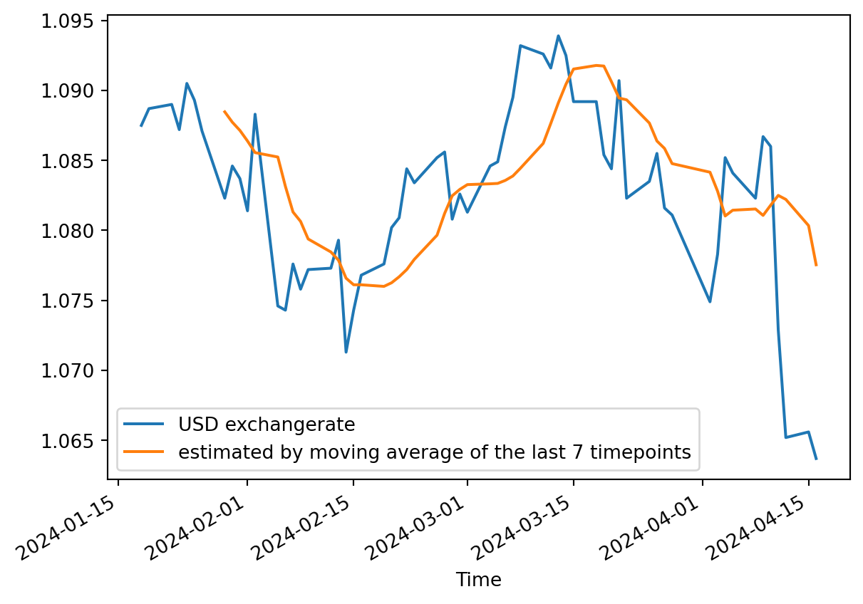
Example: predicting the current points with the average of the six previous (excluding the current point)

df['USD'].plot(label='USD exchangerate')
df['USD'].rolling(window=7, closed='left').mean().plot(
    label='estimated by moving average of the last 7 timepoints')
plt.legend()

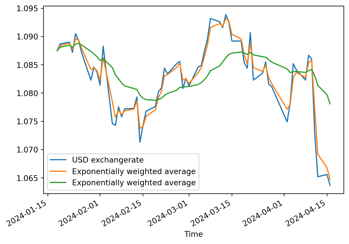
EWM: exponential moving window

only a small number of aggregation functions are implemented for exponential weighted moving avererages: https://pandas.pydata.org/docs/reference/window.html#exponentially-weighted-window-functions

df['USD'].plot(
    label='USD exchangerate')
df.USD.ewm(0.5).mean().plot(
    label='Exponentially weighted average')
df.USD.ewm(halflife='10 days', times=df.index).mean().plot(
    label='Exponentially weighted average')
plt.legend()

Group by: the ‘split’ in split-apply-combine

import seaborn as sns

penguins = sns.load_dataset("penguins")
penguins.head()

	species	island	bill_length_mm	bill_depth_mm	flipper_length_mm	body_mass_g	sex
0	Adelie	Torgersen	39.1	18.7	181.0	3750.0	Male
1	Adelie	Torgersen	39.5	17.4	186.0	3800.0	Female
2	Adelie	Torgersen	40.3	18.0	195.0	3250.0	Female
3	Adelie	Torgersen	NaN	NaN	NaN	NaN	NaN
4	Adelie	Torgersen	36.7	19.3	193.0	3450.0	Female

Iterating over groups, selecting groups

penguins.groupby('species').groups.keys()

dict_keys(['Adelie', 'Chinstrap', 'Gentoo'])

penguins.groupby('island').get_group('Dream')

	species	island	bill_length_mm	bill_depth_mm	flipper_length_mm	body_mass_g	sex
30	Adelie	Dream	39.5	16.7	178.0	3250.0	Female
31	Adelie	Dream	37.2	18.1	178.0	3900.0	Male
32	Adelie	Dream	39.5	17.8	188.0	3300.0	Female
33	Adelie	Dream	40.9	18.9	184.0	3900.0	Male
34	Adelie	Dream	36.4	17.0	195.0	3325.0	Female
...	...	...	...	...	...	...	...
215	Chinstrap	Dream	55.8	19.8	207.0	4000.0	Male
216	Chinstrap	Dream	43.5	18.1	202.0	3400.0	Female
217	Chinstrap	Dream	49.6	18.2	193.0	3775.0	Male
218	Chinstrap	Dream	50.8	19.0	210.0	4100.0	Male
219	Chinstrap	Dream	50.2	18.7	198.0	3775.0	Female

124 rows × 7 columns

grouped = penguins.groupby(['island'])

for name, df_of_group in grouped[['species', 'bill_depth_mm']]:
    print(name)
    print(df_of_group.head())

Biscoe
   species  bill_depth_mm
20  Adelie           18.3
21  Adelie           18.7
22  Adelie           19.2
23  Adelie           18.1
24  Adelie           17.2
Dream
   species  bill_depth_mm
30  Adelie           16.7
31  Adelie           18.1
32  Adelie           17.8
33  Adelie           18.9
34  Adelie           17.0
Torgersen
  species  bill_depth_mm
0  Adelie           18.7
1  Adelie           17.4
2  Adelie           18.0
3  Adelie            NaN
4  Adelie           19.3

Aggregate within groups

grouped[['bill_depth_mm', 'body_mass_g']].agg(["sum", "mean", "std"])

	bill_depth_mm			body_mass_g
	sum	mean	std	sum	mean	std
island
Biscoe	2651.1	15.874850	1.820721	787575.0	4716.017964	782.855743
Dream	2274.7	18.344355	1.133116	460400.0	3712.903226	416.644112
Torgersen	939.9	18.429412	1.339447	189025.0	3706.372549	445.107940

Aggregation with named functions, specifying specific columns

grouped.agg(
    min_depth=pd.NamedAgg(column="bill_depth_mm", aggfunc="min"),
    max_depth=pd.NamedAgg(column="bill_depth_mm", aggfunc="max"),
    average_weight=pd.NamedAgg(column="body_mass_g", aggfunc="mean"),
)

	min_depth	max_depth	average_weight
island
Biscoe	13.1	21.1	4716.017964
Dream	15.5	21.2	3712.903226
Torgersen	15.9	21.5	3706.372549

grouped.agg({
    "body_mass_g": "sum",
    "bill_depth_mm": "max"
})

	body_mass_g	bill_depth_mm
island
Biscoe	787575.0	21.1
Dream	460400.0	21.2
Torgersen	189025.0	21.5

Filtration

Filtering groups that have only very few members

penguins.shape

(344, 7)

grouped = penguins.groupby(['island'])
grouped.filter(lambda x: len(x) > 60).shape # discard groups with fewver than 60 members

(292, 7)

penguins.island.unique()

array(['Torgersen', 'Biscoe', 'Dream'], dtype=object)

grouped.filter(lambda x: len(x) > 60).island.unique() # the Torgersen was discarded

array(['Biscoe', 'Dream'], dtype=object)

(penguins.island == 'Torgersen').sum() # indeed, this is less than 60

52

Filtering out groups with missing values

def true_if_no_missing_value(x):
    return not x.isna().values.any()

df.loc['2023-11-07', 'USD'] = pd.NA
df.loc['2023-11-08', 'JPY'] = pd.NA
df.loc['2023-11-06', 'BGN'] = pd.NA
df.loc['2023-11-09', 'BGN'] = pd.NA
df.head()

	USD	JPY	BGN	CZK	DKK	GBP	CHF
Time
2024-01-18	1.0875	160.89	1.9558	24.734	7.4571	0.85773	0.9432
2024-01-19	1.0887	161.17	1.9558	24.813	7.4575	0.85825	0.9459
2024-01-22	1.0890	160.95	1.9558	24.758	7.4585	0.85575	0.9458
2024-01-23	1.0872	160.88	1.9558	24.824	7.4574	0.85493	0.9446
2024-01-24	1.0905	160.46	1.9558	24.786	7.4568	0.85543	0.9415

true_if_no_missing_value(df['CHF'])

False

true_if_no_missing_value(df['USD'])

False

penguins

	species	island	bill_length_mm	bill_depth_mm	flipper_length_mm	body_mass_g	sex
0	Adelie	Torgersen	39.1	18.7	181.0	3750.0	Male
1	Adelie	Torgersen	39.5	17.4	186.0	3800.0	Female
2	Adelie	Torgersen	40.3	18.0	195.0	3250.0	Female
3	Adelie	Torgersen	NaN	NaN	NaN	NaN	NaN
4	Adelie	Torgersen	36.7	19.3	193.0	3450.0	Female
...	...	...	...	...	...	...	...
339	Gentoo	Biscoe	NaN	NaN	NaN	NaN	NaN
340	Gentoo	Biscoe	46.8	14.3	215.0	4850.0	Female
341	Gentoo	Biscoe	50.4	15.7	222.0	5750.0	Male
342	Gentoo	Biscoe	45.2	14.8	212.0	5200.0	Female
343	Gentoo	Biscoe	49.9	16.1	213.0	5400.0	Male

344 rows × 7 columns

penguins.loc[0, 'body_mass_g'] = pd.NA
penguins.head()

	species	island	bill_length_mm	bill_depth_mm	flipper_length_mm	body_mass_g	sex
0	Adelie	Torgersen	39.1	18.7	181.0	NaN	Male
1	Adelie	Torgersen	39.5	17.4	186.0	3800.0	Female
2	Adelie	Torgersen	40.3	18.0	195.0	3250.0	Female
3	Adelie	Torgersen	NaN	NaN	NaN	NaN	NaN
4	Adelie	Torgersen	36.7	19.3	193.0	3450.0	Female

Filtering any groups that have a missing value

grouped['body_mass_g'].filter(lambda s: true_if_no_missing_value(s))

30     3250.0
31     3900.0
32     3300.0
33     3900.0
34     3325.0
        ...  
215    4000.0
216    3400.0
217    3775.0
218    4100.0
219    3775.0
Name: body_mass_g, Length: 124, dtype: float64

# discard groups with any missing value in body_mass_g or bill_length_mm columns
grouped.filter(lambda d: true_if_no_missing_value(d['body_mass_g']) and
                         true_if_no_missing_value(d['bill_length_mm']))

	species	island	bill_length_mm	bill_depth_mm	flipper_length_mm	body_mass_g	sex
30	Adelie	Dream	39.5	16.7	178.0	3250.0	Female
31	Adelie	Dream	37.2	18.1	178.0	3900.0	Male
32	Adelie	Dream	39.5	17.8	188.0	3300.0	Female
33	Adelie	Dream	40.9	18.9	184.0	3900.0	Male
34	Adelie	Dream	36.4	17.0	195.0	3325.0	Female
...	...	...	...	...	...	...	...
215	Chinstrap	Dream	55.8	19.8	207.0	4000.0	Male
216	Chinstrap	Dream	43.5	18.1	202.0	3400.0	Female
217	Chinstrap	Dream	49.6	18.2	193.0	3775.0	Male
218	Chinstrap	Dream	50.8	19.0	210.0	4100.0	Male
219	Chinstrap	Dream	50.2	18.7	198.0	3775.0	Female

124 rows × 7 columns

Transformation: assign the group average for missing values

grouped['body_mass_g'].transform(lambda x: x.fillna(value=x.mean()))

0      3705.500000
1      3800.000000
2      3250.000000
3      3705.500000
4      3450.000000
          ...     
339    4716.017964
340    4850.000000
341    5750.000000
342    5200.000000
343    5400.000000
Name: body_mass_g, Length: 344, dtype: float64

grouped['body_mass_g'].agg('mean')

island
Biscoe       4716.017964
Dream        3712.903226
Torgersen    3705.500000
Name: body_mass_g, dtype: float64

from pandas.api.types import is_numeric_dtype
# impute the mean, over each group, for all numeric columns
grouped.transform(lambda x: x.fillna(value=x.mean()) if is_numeric_dtype(x) else x)

	species	bill_length_mm	bill_depth_mm	flipper_length_mm	body_mass_g	sex
0	Adelie	39.100000	18.700000	181.000000	3705.500000	Male
1	Adelie	39.500000	17.400000	186.000000	3800.000000	Female
2	Adelie	40.300000	18.000000	195.000000	3250.000000	Female
3	Adelie	38.950980	18.429412	191.196078	3705.500000	NaN
4	Adelie	36.700000	19.300000	193.000000	3450.000000	Female
...	...	...	...	...	...	...
339	Gentoo	45.257485	15.874850	209.706587	4716.017964	NaN
340	Gentoo	46.800000	14.300000	215.000000	4850.000000	Female
341	Gentoo	50.400000	15.700000	222.000000	5750.000000	Male
342	Gentoo	45.200000	14.800000	212.000000	5200.000000	Female
343	Gentoo	49.900000	16.100000	213.000000	5400.000000	Male

344 rows × 6 columns