Lec 13 - Enriching your dataframe with external information and join/merge

import seaborn as sns
import pandas as pd

# This is a comment in python
# Another comment

penguins = sns.load_dataset('penguins')
penguins.head()
species island bill_length_mm bill_depth_mm flipper_length_mm body_mass_g sex
0 Adelie Torgersen 39.1 18.7 181.0 3750.0 Male
1 Adelie Torgersen 39.5 17.4 186.0 3800.0 Female
2 Adelie Torgersen 40.3 18.0 195.0 3250.0 Female
3 Adelie Torgersen NaN NaN NaN NaN NaN
4 Adelie Torgersen 36.7 19.3 193.0 3450.0 Female
# third comment

geo_df = pd.DataFrame([
    {'island name': 'Torgersen', 'lat': -64.766667, 'lon': -64.083333},
    {'island name': 'Biscoe', 'lat': -65.4333, 'lon': -65.5000},
    {'island name': 'Dream', 'lat':  -64.7333, 'lon': -64.2333}
    ])
geo_df
island name lat lon
0 Torgersen -64.766667 -64.083333
1 Biscoe -65.433300 -65.500000
2 Dream -64.733300 -64.233300
import plotly.express as px
fig = px.scatter_geo(geo_df,
                     lat='lat', lon='lon',
                     hover_name="island name",
                     fitbounds="locations")

fig.show()
merged_df = penguins.merge(geo_df, left_on='island', right_on='island name')
merged_df.head()
species island bill_length_mm bill_depth_mm flipper_length_mm body_mass_g sex island name lat lon
0 Adelie Torgersen 39.1 18.7 181.0 3750.0 Male Torgersen -64.766667 -64.083333
1 Adelie Torgersen 39.5 17.4 186.0 3800.0 Female Torgersen -64.766667 -64.083333
2 Adelie Torgersen 40.3 18.0 195.0 3250.0 Female Torgersen -64.766667 -64.083333
3 Adelie Torgersen NaN NaN NaN NaN NaN Torgersen -64.766667 -64.083333
4 Adelie Torgersen 36.7 19.3 193.0 3450.0 Female Torgersen -64.766667 -64.083333
df_agg = merged_df.groupby('island')[['body_mass_g', 'flipper_length_mm', 'lat', 'lon']].agg('mean')
df_agg
body_mass_g flipper_length_mm lat lon
island
Biscoe 4716.017964 209.706587 -65.433300 -65.500000
Dream 3712.903226 193.072581 -64.733300 -64.233300
Torgersen 3706.372549 191.196078 -64.766667 -64.083333
df_agg['island'] = df_agg.index
fig = px.scatter_geo(df_agg,
                     lat='lat', lon='lon',
                     size='body_mass_g',
                     color='flipper_length_mm',
                     hover_name="island",
                     fitbounds="locations")

fig.show()

Different types of join

# Little helper to print dataframes side by side
# https://stackoverflow.com/a/44923103/13430450
from IPython.display import display_html
from itertools import chain,cycle
def display_side_by_side(*args,titles=cycle([''])):
    html_str=''
    for df,title in zip(args, chain(titles,cycle(['</br>'])) ):
        html_str+='<th style="text-align:center"><td style="vertical-align:top">'
        html_str+=f'<h2 style="text-align: center;">{title}</h2>'
        html_str+=df.to_html().replace('table','table style="display:inline"')
        html_str+='</td></th>'
    display_html(html_str,raw=True)
left = pd.DataFrame(
    {
        "key": ["K0", "K1", "K2", "K3"],
        "A": ["A0", "A1", "A2", "A3"],
        "B": ["B0", "B1", "B2", "B3"],
    })
right = pd.DataFrame(
    {
        "key": ["K0", "K1", "K2", "K3"],
        "C": ["C0", "C1", "C2", "C3"],
        "D": ["D0", "D1", "D2", "D3"],
    })
display_side_by_side(left,
                     right,
                     pd.merge(left, right, on="key", indicator=True),
                     titles=['left', 'right', 'merged'])

left

key A B
0 K0 A0 B0
1 K1 A1 B1
2 K2 A2 B2
3 K3 A3 B3

right

key C D
0 K0 C0 D0
1 K1 C1 D1
2 K2 C2 D2
3 K3 C3 D3

merged

key A B C D _merge
0 K0 A0 B0 C0 D0 both
1 K1 A1 B1 C1 D1 both
2 K2 A2 B2 C2 D2 both
3 K3 A3 B3 C3 D3 both

Left merge: Use keys from left frame only (in SQL, “LEFT OUTER JOIN”)

left = pd.DataFrame(
    {
        "key1": ["K0", "K0", "K1", "K2"],
        "key2": ["K0", "K1", "K0", "K1"],
        "A": ["A0", "A1", "A2", "A3"],
        "B": ["B0", "B1", "B2", "B3"],
    }
)
right = pd.DataFrame(
    {
        "key1": ["K0", "K1", "K1", "K2"],
        "key2": ["K0", "K0", "K0", "K0"],
        "C": ["C0", "C1", "C2", "C3"],
        "D": ["D0", "D1", "D2", "D3"],
    }
)
display_side_by_side(left,
                     right,
                     pd.merge(left,
                              right,
                              how="left",
                              on=["key1", "key2"],
                              indicator=True
                              ),
                     titles=['left', 'right', 'merged (how=left)'])

left

key1 key2 A B
0 K0 K0 A0 B0
1 K0 K1 A1 B1
2 K1 K0 A2 B2
3 K2 K1 A3 B3

right

key1 key2 C D
0 K0 K0 C0 D0
1 K1 K0 C1 D1
2 K1 K0 C2 D2
3 K2 K0 C3 D3

merged (how=left)

key1 key2 A B C D _merge
0 K0 K0 A0 B0 C0 D0 both
1 K0 K1 A1 B1 NaN NaN left_only
2 K1 K0 A2 B2 C1 D1 both
3 K1 K0 A2 B2 C2 D2 both
4 K2 K1 A3 B3 NaN NaN left_only

Right merge: Use keys from right frame only (in SQL, “RIGHT OUTER JOIN”)

display_side_by_side(left,
                     right,
                     pd.merge(left, right, how="right", on=["key1", "key2"], indicator=True),
                     titles=['left', 'right', 'merged (how=right)'])

left

key1 key2 A B
0 K0 K0 A0 B0
1 K0 K1 A1 B1
2 K1 K0 A2 B2
3 K2 K1 A3 B3

right

key1 key2 C D
0 K0 K0 C0 D0
1 K1 K0 C1 D1
2 K1 K0 C2 D2
3 K2 K0 C3 D3

merged (how=right)

key1 key2 A B C D _merge
0 K0 K0 A0 B0 C0 D0 both
1 K1 K0 A2 B2 C1 D1 both
2 K1 K0 A2 B2 C2 D2 both
3 K2 K0 NaN NaN C3 D3 right_only

Outer join: Use union of keys from both frames (“in SQL,”FULL OUTER JOIN”)

display_side_by_side(left,
                     right,
                     pd.merge(left, right, how="outer", on=["key1", "key2"],  indicator=True),
                     titles=['left', 'right', 'merged (how=outer)'])

left

key1 key2 A B
0 K0 K0 A0 B0
1 K0 K1 A1 B1
2 K1 K0 A2 B2
3 K2 K1 A3 B3

right

key1 key2 C D
0 K0 K0 C0 D0
1 K1 K0 C1 D1
2 K1 K0 C2 D2
3 K2 K0 C3 D3

merged (how=outer)

key1 key2 A B C D _merge
0 K0 K0 A0 B0 C0 D0 both
1 K0 K1 A1 B1 NaN NaN left_only
2 K1 K0 A2 B2 C1 D1 both
3 K1 K0 A2 B2 C2 D2 both
4 K2 K1 A3 B3 NaN NaN left_only
5 K2 K0 NaN NaN C3 D3 right_only

Inner join: Use intersection of keys from both frames (in SQL, “INNER JOIN”)

display_side_by_side(left,
                     right,
                     pd.merge(left, right, how="inner", on=["key1", "key2"], indicator=True),
                     titles=['left', 'right', 'merged (how=inner)'])

left

key1 key2 A B
0 K0 K0 A0 B0
1 K0 K1 A1 B1
2 K1 K0 A2 B2
3 K2 K1 A3 B3

right

key1 key2 C D
0 K0 K0 C0 D0
1 K1 K0 C1 D1
2 K1 K0 C2 D2
3 K2 K0 C3 D3

merged (how=inner)

key1 key2 A B C D _merge
0 K0 K0 A0 B0 C0 D0 both
1 K1 K0 A2 B2 C1 D1 both
2 K1 K0 A2 B2 C2 D2 both

how='cross': Create the cartesian product of rows of both frames

display_side_by_side(left,
                     right,
                     pd.merge(left, right, how="cross", suffixes=('_x', '_y')),                     
                     titles=['left', 'right', 'merged (how=cross)'])

left

key1 key2 A B
0 K0 K0 A0 B0
1 K0 K1 A1 B1
2 K1 K0 A2 B2
3 K2 K1 A3 B3

right

key1 key2 C D
0 K0 K0 C0 D0
1 K1 K0 C1 D1
2 K1 K0 C2 D2
3 K2 K0 C3 D3

merged (how=cross)

key1_x key2_x A B key1_y key2_y C D
0 K0 K0 A0 B0 K0 K0 C0 D0
1 K0 K0 A0 B0 K1 K0 C1 D1
2 K0 K0 A0 B0 K1 K0 C2 D2
3 K0 K0 A0 B0 K2 K0 C3 D3
4 K0 K1 A1 B1 K0 K0 C0 D0
5 K0 K1 A1 B1 K1 K0 C1 D1
6 K0 K1 A1 B1 K1 K0 C2 D2
7 K0 K1 A1 B1 K2 K0 C3 D3
8 K1 K0 A2 B2 K0 K0 C0 D0
9 K1 K0 A2 B2 K1 K0 C1 D1
10 K1 K0 A2 B2 K1 K0 C2 D2
11 K1 K0 A2 B2 K2 K0 C3 D3
12 K2 K1 A3 B3 K0 K0 C0 D0
13 K2 K1 A3 B3 K1 K0 C1 D1
14 K2 K1 A3 B3 K1 K0 C2 D2
15 K2 K1 A3 B3 K2 K0 C3 D3

Another application: Enrich our forex rates dataframe with market data

rates = pd.read_csv('rates.csv', parse_dates=['Time'])
rates.head()
Time USD JPY BGN CZK DKK GBP CHF
0 2024-04-16 1.0637 164.54 1.9558 25.210 7.4609 0.85440 0.9712
1 2024-04-15 1.0656 164.05 1.9558 25.324 7.4606 0.85405 0.9725
2 2024-04-12 1.0652 163.16 1.9558 25.337 7.4603 0.85424 0.9716
3 2024-04-11 1.0729 164.18 1.9558 25.392 7.4604 0.85525 0.9787
4 2024-04-10 1.0860 164.89 1.9558 25.368 7.4594 0.85515 0.9810
import yfinance as yf

msft = yf.Ticker("MSFT")
msft.info
msft_hist = msft.history(period="6mo")
msft_hist.head()
Open High Low Close Volume Dividends Stock Splits
Date
2023-10-23 00:00:00-04:00 324.211180 331.443110 323.135370 328.046295 24374700 0.0 0.0
2023-10-24 00:00:00-04:00 330.018628 330.556548 326.332957 329.251617 31153600 0.0 0.0
2023-10-25 00:00:00-04:00 343.685568 344.861028 336.314195 339.352417 55053800 0.0 0.0
2023-10-26 00:00:00-04:00 339.222925 340.308706 325.675519 326.621857 37828500 0.0 0.0
2023-10-27 00:00:00-04:00 329.152021 335.417702 327.129873 328.534424 29856500 0.0 0.0
# create a column for date only (without timezone/hours/minutes/seconds)
msft_hist['date_only'] = pd.to_datetime(msft_hist.index.date)
msft_hist.head()
Open High Low Close Volume Dividends Stock Splits date_only
Date
2023-10-23 00:00:00-04:00 324.211180 331.443110 323.135370 328.046295 24374700 0.0 0.0 2023-10-23
2023-10-24 00:00:00-04:00 330.018628 330.556548 326.332957 329.251617 31153600 0.0 0.0 2023-10-24
2023-10-25 00:00:00-04:00 343.685568 344.861028 336.314195 339.352417 55053800 0.0 0.0 2023-10-25
2023-10-26 00:00:00-04:00 339.222925 340.308706 325.675519 326.621857 37828500 0.0 0.0 2023-10-26
2023-10-27 00:00:00-04:00 329.152021 335.417702 327.129873 328.534424 29856500 0.0 0.0 2023-10-27
spy = yf.Ticker("SPY")
spy.info
spy_hist = spy.history(period="6mo")
spy_hist.head()
Open High Low Close Volume Dividends Stock Splits Capital Gains
Date
2023-10-23 00:00:00-04:00 416.621136 421.426688 414.824031 417.465088 92035100 0.0 0.0 0.0
2023-10-24 00:00:00-04:00 419.639488 421.794044 417.743089 420.612518 78564200 0.0 0.0 0.0
2023-10-25 00:00:00-04:00 418.884919 418.914704 414.049582 414.575806 94223200 0.0 0.0 0.0
2023-10-26 00:00:00-04:00 413.483664 414.357371 408.668205 409.611420 115156800 0.0 0.0 0.0
2023-10-27 00:00:00-04:00 411.239769 411.646852 406.295230 407.754761 107367700 0.0 0.0 0.0
# create a column for date only (without timezone/hours/minutes/seconds)

spy_hist['date_only'] = pd.to_datetime(spy_hist.index.date)
spy_hist.head()
Open High Low Close Volume Dividends Stock Splits Capital Gains date_only
Date
2023-10-23 00:00:00-04:00 416.621136 421.426688 414.824031 417.465088 92035100 0.0 0.0 0.0 2023-10-23
2023-10-24 00:00:00-04:00 419.639488 421.794044 417.743089 420.612518 78564200 0.0 0.0 0.0 2023-10-24
2023-10-25 00:00:00-04:00 418.884919 418.914704 414.049582 414.575806 94223200 0.0 0.0 0.0 2023-10-25
2023-10-26 00:00:00-04:00 413.483664 414.357371 408.668205 409.611420 115156800 0.0 0.0 0.0 2023-10-26
2023-10-27 00:00:00-04:00 411.239769 411.646852 406.295230 407.754761 107367700 0.0 0.0 0.0 2023-10-27
df_with_spy = rates.merge(spy_hist[['date_only', 'Close']],
                          how='left',
                          left_on='Time',
                          right_on='date_only')
df_with_spy.columns = ['Time', 'USD', 'JPY', 'BGN', 'CZK', 'DKK', 'GBP', 'CHF', 'date_only',
       'Close_spy']
df_with_spy
Time USD JPY BGN CZK DKK GBP CHF date_only Close_spy
0 2024-04-16 1.0637 164.54 1.9558 25.210 7.4609 0.85440 0.9712 2024-04-16 503.529999
1 2024-04-15 1.0656 164.05 1.9558 25.324 7.4606 0.85405 0.9725 2024-04-15 504.450012
2 2024-04-12 1.0652 163.16 1.9558 25.337 7.4603 0.85424 0.9716 2024-04-12 510.850006
3 2024-04-11 1.0729 164.18 1.9558 25.392 7.4604 0.85525 0.9787 2024-04-11 518.000000
4 2024-04-10 1.0860 164.89 1.9558 25.368 7.4594 0.85515 0.9810 2024-04-10 514.119995
... ... ... ... ... ... ... ... ... ... ...
57 2024-01-24 1.0905 160.46 1.9558 24.786 7.4568 0.85543 0.9415 2024-01-24 483.886566
58 2024-01-23 1.0872 160.88 1.9558 24.824 7.4574 0.85493 0.9446 2024-01-23 483.358185
59 2024-01-22 1.0890 160.95 1.9558 24.758 7.4585 0.85575 0.9458 2024-01-22 481.952576
60 2024-01-19 1.0887 161.17 1.9558 24.813 7.4575 0.85825 0.9459 2024-01-19 480.935699
61 2024-01-18 1.0875 160.89 1.9558 24.734 7.4571 0.85773 0.9432 2024-01-18 475.014099

62 rows × 10 columns

df_with_spy_with_msft = df_with_spy.merge(msft_hist[['date_only', 'Close']], on='date_only')
df_with_spy_with_msft.columns = ['Time', 'USD', 'JPY', 'BGN', 'CZK', 'DKK', 'GBP', 'CHF', 'date_only',
       'Close_spy', 'Close_MSFT']
df_with_spy_with_msft.head()
Time USD JPY BGN CZK DKK GBP CHF date_only Close_spy Close_MSFT
0 2024-04-16 1.0637 164.54 1.9558 25.210 7.4609 0.85440 0.9712 2024-04-16 503.529999 414.579987
1 2024-04-15 1.0656 164.05 1.9558 25.324 7.4606 0.85405 0.9725 2024-04-15 504.450012 413.640015
2 2024-04-12 1.0652 163.16 1.9558 25.337 7.4603 0.85424 0.9716 2024-04-12 510.850006 421.899994
3 2024-04-11 1.0729 164.18 1.9558 25.392 7.4604 0.85525 0.9787 2024-04-11 518.000000 427.929993
4 2024-04-10 1.0860 164.89 1.9558 25.368 7.4594 0.85515 0.9810 2024-04-10 514.119995 423.260010
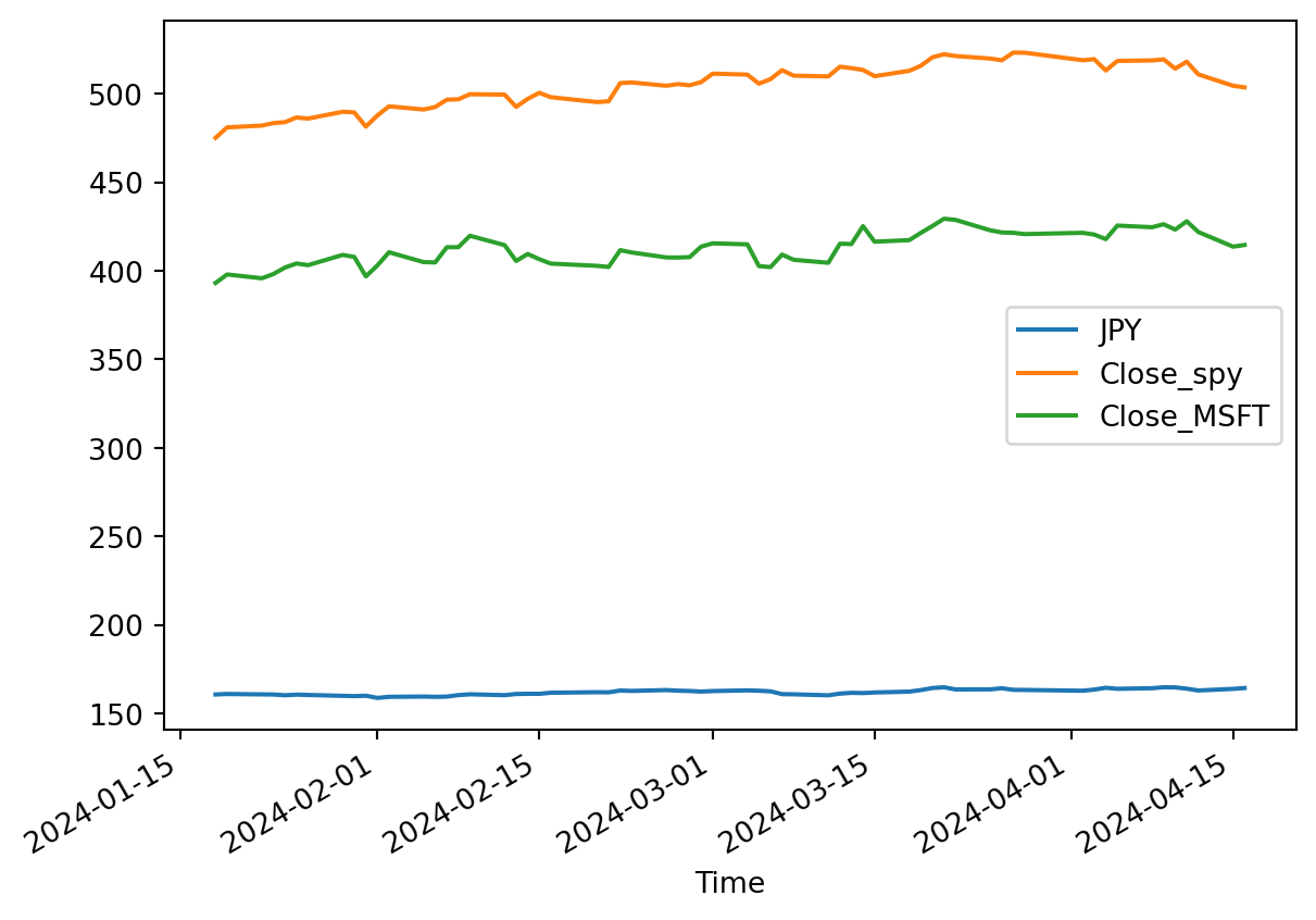
from matplotlib import pyplot as plt

ax = plt.gca()
df_with_spy_with_msft.plot(x='Time', y='JPY', ax=ax)
df_with_spy_with_msft.plot(x='Time', y='Close_spy', ax=ax)
df_with_spy_with_msft.plot(x='Time', y='Close_MSFT', ax=ax)

NYC flights data: plot destination airports with marker size proportional to the number of flights to a particular airports

from nycflights13 import flights, airports, airlines, planes, weather
flights.head()
year month day dep_time sched_dep_time dep_delay arr_time sched_arr_time arr_delay carrier flight tailnum origin dest air_time distance hour minute time_hour
0 2013 1 1 517.0 515 2.0 830.0 819 11.0 UA 1545 N14228 EWR IAH 227.0 1400 5 15 2013-01-01T10:00:00Z
1 2013 1 1 533.0 529 4.0 850.0 830 20.0 UA 1714 N24211 LGA IAH 227.0 1416 5 29 2013-01-01T10:00:00Z
2 2013 1 1 542.0 540 2.0 923.0 850 33.0 AA 1141 N619AA JFK MIA 160.0 1089 5 40 2013-01-01T10:00:00Z
3 2013 1 1 544.0 545 -1.0 1004.0 1022 -18.0 B6 725 N804JB JFK BQN 183.0 1576 5 45 2013-01-01T10:00:00Z
4 2013 1 1 554.0 600 -6.0 812.0 837 -25.0 DL 461 N668DN LGA ATL 116.0 762 6 0 2013-01-01T11:00:00Z
airports.head()
faa name lat lon alt tz dst tzone
0 04G Lansdowne Airport 41.130472 -80.619583 1044 -5 A America/New_York
1 06A Moton Field Municipal Airport 32.460572 -85.680028 264 -6 A America/Chicago
2 06C Schaumburg Regional 41.989341 -88.101243 801 -6 A America/Chicago
3 06N Randall Airport 41.431912 -74.391561 523 -5 A America/New_York
4 09J Jekyll Island Airport 31.074472 -81.427778 11 -5 A America/New_York
planes.head()
tailnum year type manufacturer model engines seats speed engine
0 N10156 2004.0 Fixed wing multi engine EMBRAER EMB-145XR 2 55 NaN Turbo-fan
1 N102UW 1998.0 Fixed wing multi engine AIRBUS INDUSTRIE A320-214 2 182 NaN Turbo-fan
2 N103US 1999.0 Fixed wing multi engine AIRBUS INDUSTRIE A320-214 2 182 NaN Turbo-fan
3 N104UW 1999.0 Fixed wing multi engine AIRBUS INDUSTRIE A320-214 2 182 NaN Turbo-fan
4 N10575 2002.0 Fixed wing multi engine EMBRAER EMB-145LR 2 55 NaN Turbo-fan
airlines.head()
carrier name
0 9E Endeavor Air Inc.
1 AA American Airlines Inc.
2 AS Alaska Airlines Inc.
3 B6 JetBlue Airways
4 DL Delta Air Lines Inc.
weather.head()
origin year month day hour temp dewp humid wind_dir wind_speed wind_gust precip pressure visib time_hour
0 EWR 2013 1 1 1 39.02 26.06 59.37 270.0 10.35702 NaN 0.0 1012.0 10.0 2013-01-01T06:00:00Z
1 EWR 2013 1 1 2 39.02 26.96 61.63 250.0 8.05546 NaN 0.0 1012.3 10.0 2013-01-01T07:00:00Z
2 EWR 2013 1 1 3 39.02 28.04 64.43 240.0 11.50780 NaN 0.0 1012.5 10.0 2013-01-01T08:00:00Z
3 EWR 2013 1 1 4 39.92 28.04 62.21 250.0 12.65858 NaN 0.0 1012.2 10.0 2013-01-01T09:00:00Z
4 EWR 2013 1 1 5 39.02 28.04 64.43 260.0 12.65858 NaN 0.0 1011.9 10.0 2013-01-01T10:00:00Z
# count number of flights per airport
series_number_of_flights = flights[['dest']].groupby('dest').size()
series_number_of_flights.name = 'Count flights'
series_number_of_flights
dest
ABQ      254
ACK      265
ALB      439
ANC        8
ATL    17215
       ...  
TPA     7466
TUL      315
TVC      101
TYS      631
XNA     1036
Name: Count flights, Length: 105, dtype: int64
airports_with_flight_counts = airports.merge(series_number_of_flights,
                                            left_on='faa',
                                            right_index=True)
airports_with_flight_counts
faa name lat lon alt tz dst tzone Count flights
87 ABQ Albuquerque International Sunport 35.040222 -106.609194 5355 -7 A America/Denver 254
91 ACK Nantucket Mem 41.253053 -70.060181 48 -5 A America/New_York 265
118 ALB Albany Intl 42.748267 -73.801692 285 -5 A America/New_York 439
128 ANC Ted Stevens Anchorage Intl 61.174361 -149.996361 152 -9 A America/Anchorage 8
153 ATL Hartsfield Jackson Atlanta Intl 33.636719 -84.428067 1026 -5 A America/New_York 17215
... ... ... ... ... ... ... ... ... ...
1327 TPA Tampa Intl 27.975472 -82.533250 26 -5 A America/New_York 7466
1334 TUL Tulsa Intl 36.198389 -95.888111 677 -6 A America/Chicago 315
1337 TVC Cherry Capital Airport 44.741445 -85.582235 624 -5 A America/New_York 101
1347 TYS Mc Ghee Tyson 35.810972 -83.994028 981 -5 A America/New_York 631
1430 XNA NW Arkansas Regional 36.281869 -94.306811 1287 -6 A America/Chicago 1036

101 rows × 9 columns

# SFO and LAX (large airport)
airports_with_flight_counts.query('faa == "LAX" or faa == "SFO"')
faa name lat lon alt tz dst tzone Count flights
770 LAX Los Angeles Intl 33.942536 -118.408075 126 -8 A America/Los_Angeles 16174
1216 SFO San Francisco Intl 37.618972 -122.374889 13 -8 A America/Los_Angeles 13331
fig = px.scatter_geo(airports_with_flight_counts,
                     lat='lat', lon='lon',
                     hover_name="name",
                     fitbounds="locations",
                     size='Count flights'
                    )
fig.show()
series_airport_with_mean_delay = flights[['dest', 'dep_delay']].groupby('dest').mean()
series_airport_with_mean_delay.name = 'delay'
series_airport_with_mean_delay.head()
dep_delay
dest
ABQ 13.740157
ACK 6.456604
ALB 23.620525
ANC 12.875000
ATL 12.509824
airports_with_flight_counts_with_delays = airports.merge(
    series_number_of_flights,
    left_on='faa',
    right_index=True
).merge(
        series_airport_with_mean_delay,
        left_on='faa',
        right_index=True
)
airports_with_flight_counts_with_delays.query('faa == "LAX" or faa == "SFO"')
faa name lat lon alt tz dst tzone Count flights dep_delay
770 LAX Los Angeles Intl 33.942536 -118.408075 126 -8 A America/Los_Angeles 16174 9.401344
1216 SFO San Francisco Intl 37.618972 -122.374889 13 -8 A America/Los_Angeles 13331 12.866289
fig = px.scatter_geo(airports_with_flight_counts_with_delays,
                     lat='lat', lon='lon',
                     hover_name="name",
                     fitbounds="locations",
                     size='Count flights',
                     color='dep_delay'
                    )
fig.show()